Séance 4, 5-Instruments for pollution control

How to choose the instrument?

Market allocation of pollution

• Air and water are treated in our legal system as common-pool resources, and as such the market misallocates them.
• Pollutant damages are commonly externalities.
  • These costs are not borne by the emitting source and hence not considered by it, although they certainly are borne by society at large.
• With pollution, as this cost is borne partially by the society rather than producers, it does not find its way into product prices.
• Not only does the unimpeded market fail to generate the efficient level of pollution control, but also it penalises those firms that might attempt to control an efficient amount.
• Government intervention is particularly needed for pollution control.

Efficient policy responses

• For a market as a whole, efficiency is achieved when the marginal cost of control is equal to the marginal damage caused by the pollution.
  • However, markets often fail to produce an efficient level of pollution.
• An alternative approach would be to internalise the marginal damage caused by each unit of emissions by means of a tax or charge on each unit of emissions.
  • This per-unit charge could increase with the level of pollution or the tax rate could be constant as long as the rate were equal to the marginal social damage at the point where the marginal social damage and marginal control costs cross.
  • Since the emitter is paying the marginal social damage when confronted by these fees, pollution costs would be internalised.

How to choose an instrument?

• One approach is to select specific legal levels of pollution based on some other criterion, such as providing adequate margins of safety for human or ecological health.
  • Different countries have different criteria for what an adequate margin represents.
• How an Environmental Protection Agency (EPA) could attain a predetermined pollution target?
  • What instruments that could be used.
  • Depends on what criteria.
• Multitude of instruments in fact.
• Main question: which is the best instrument ?
• There are many instruments available to an EPA charged with attaining some pollution target.
• The best instrument would be the one which meets the target with greatest reliability.
• But the EPA is unlikely to have only this objective.
  • Government typically has multiple objectives, and the terms of reference that policy makers impose on their agents will tend to reflect that diversity of objectives.

Choice based on the above

Instrument choice can be envisaged in the following way:

• Each available instrument can be characterised by a set of attributes, relating to such things as impacts on income and wealth distribution, the structure of incentives generated, and the costs imposed in abating pollution.
• A score can be given to each instrument, dependent on how well its attributes match with the set of objectives sought by the EPA.
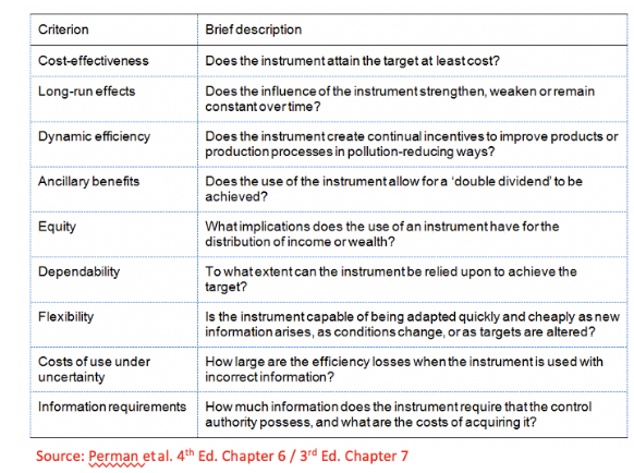
• The table in the next slide lays out a set of criteria in terms of which the relative merits of instruments can be assessed.

Criteria for choice of pollution control instruments

Cost efficiency and cost-effective pollution abatement instruments

• Suppose a list is available of all instruments which are capable of achieving some predetermined pollution abatement target.
• If one particular instrument can attain that target at lower real cost than any other can then that instrument is cost-effective.
• Cost-effectiveness is clearly a desirable attribute of an instrument:
  • Using a cost-effective instrument involves allocating the smallest amount of resources to pollution control, conditional on a given target being achieved.
  • It has the minimum opportunity cost.
  • Hence, the use of cost-effective instruments is a prerequisite for achieving an economically efficient allocation of resources.

Practical application

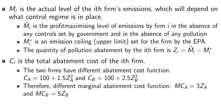
• Suppose government wishes to reduce the total emission of a particular pollutant from the current, uncontrolled, level ˆM (say, 90 units per period) to a target level M* (say, 50 units), which means 40 units of emission per period.
• Emissions arise from the activities of two firms, A (40 units) and B (50 units).
• The principle of cost efficiency provides a very clear answer: a necessary condition for abatement at least cost is that the marginal cost of abatement be equalised over all abaters.
  • This result is known as the least cost theorem of pollution control. Marginal cost→derivative of cost.

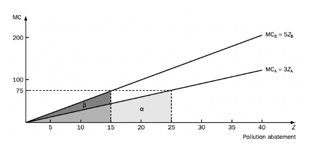
Graphical representation

Conclusion

The least-cost solution is obtained by finding levels of ZA and ZB which add up to the overall abatement target Z = 40 and which satisfy the least-cost condition that MCA = MCB:

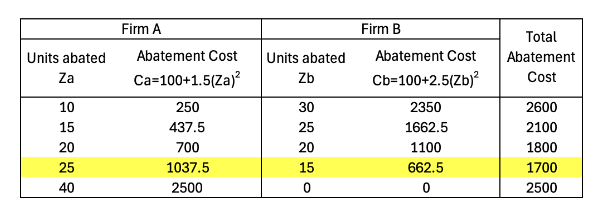
• Figure in the previous slide shows this least cost solution is where both firms have marginal abatement costs of 75.
• Minimised total abatement costs (1700) can be read from the diagram. B’s total abatement; B’s total abatement costs (662.5), A’s total abatement costs (1037.5).
• A least-cost control regime implies that the marginal cost of abatement is equalised over all firms undertaking pollution control.
• A least-cost solution will in general not involve equal abatement effort by all polluters.
• Where abatement costs differ, cost efficiency implies that relatively low-cost abaters will undertake most of the total abatement effort, but not usually all of it.

Comparing this solution with two others…

1. One might think that as firm A has a lower marginal abatement cost schedule than B it should undertake all 40 units of abatement.
   • It is easy to verify that this results in higher costs (2500) than those found in the least-cost solution (1700).
2. An equity argument might be invoked to justify sharing the abatement burden equally between the two firms.
   • it is easy to show that this also leads to higher costs (1800 in fact).

Overview of instruments for achieving pollution abatement targets

• Institutional approaches which facilitate internalisation of externalities:
  • Bargaining solutions.
  • Liability.
  • Development of social responsibility.
• Command and control (CAC) instruments:
  • Non-transferable emissions licences.
  • Instruments which impose minimum technology requirements.
  • Location.
• Economic incentive (quasi-market) instruments:
  • Emissions taxes.
  • Pollution abatement subsidies.
  • Marketable emissions permits.

Taxes

• First proposed by Arthur Pigou (1938), taxes are one of the most commonly advocated instruments by economists to address environmental externalities.
• Increasingly used, especially in areas like waste disposal and for the control of specific air and water pollutants.
• Two main types:
  • Emission taxes: levied on the pollutant itself (tax on SO2 emissions);
  • Product charges: levied on final products (taxes on fuels or pesticides).

Basic idea

• General approach: allows entities to emit as much pollution as they wish, but must pay a fixed price per unit of emission (or output).
• Polluter pays principle: Intuitively fair.

How much pollution control would the firm choose? Practical example

• The level of uncontrolled emission is 15 units and the emissions charge is T:
  • If the firm were to decide against controlling any emissions, it would have to pay T times 15, represented by area 0TBC.
• Is this the best the firm can do?
  • Obviously not, since it can control some pollution at a lower cost than paying the emissions charge.
  • It would pay the firm to reduce emissions until the marginal cost of reduction is equal to the emissions charge.
• The firm would minimise its cost by choosing to clean up ten units of pollution and to emit five units.
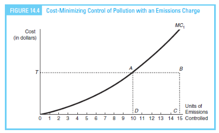
  • At this allocation the firm would pay control costs equal to area 0AD and total emissions charge payments equal to area ABCD.

Numerical example

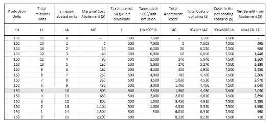
Key results

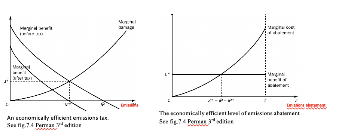
• The tax instrument - at rate μ - brings about a socially efficient aggregate level of pollution.
• Given this, the post-tax marginal benefit schedule differs from its pre-tax counterpart by that value of marginal damage.
• Once the tax is operative, profit maximising behaviour by firms leads to a pollution choice of M∗, rather than ˆM as was before the tax.
• An emission tax at rate μ∗ creates just the right amount of incentive to bring about the targeted efficient emission level.
• In the absence of an emissions tax (or an abatement subsidy), firms have no economic incentive to abate pollution,
• When an emissions tax is levied (or, equivalently, when an abatement subsidy is available) an incentive to abate exists in the form of tax avoided (or subsidy gained).
• It will be profitable for firms to reduce pollution as long as their marginal abatement costs are less than the value of the tax rate per unit of pollution.
• The efficient pollution level is attained without coercion, purely as a result of the altered structure of incentives facing firms.
• The tax eliminates the wedge (created by pollution damage) between private and socially efficient prices.
• The tax brings private prices of emissions (zero) into line with social prices μ∗.
• The tax ‘internalises the externality’ by inducing the pollution generator to behave as if pollution costs entered its private cost functions.
• Not only will the tax instrument bring about an efficient level of pollution but it will also achieve that target in a cost-effective way.
  • Remember that cost-efficiency requires that the marginal abatement cost be equal over all abaters.
  • All firms adjust their firm-specific abatement levels to equate their marginal abatement cost with the tax rate.
  • As the tax rate is identical for all firms, so are their marginal costs.
  • The only issue here is that it isn’t always easy to identify the adequate tax value. It would require to put together the marginal cost of emmission abatement of each firm. Provided that our regulator know the marginal cost of abatement he would be able to identify the correct tax value.
• To attain the economically efficient level of emissions M∗, knowledge of the aggregate (economy-wide) marginal emissions abatement cost function would be sufficient.
• For any target ˜M, knowledge of the aggregate marginal cost of abatement function allows the EPA to identify the tax rate, say ˜μ, that would create the right incentive to bring about that outcome.
• The emissions tax, levied at ˜μ, attains the target ˜M at least total cost, and so is cost efficient.
• Not only does the EPA not need to know the aggregate marginal pollution damage function, it does not need to know the abatement cost function of each firm.

Subsidies

• Carrot vs. Stick.
• Society pays polluter to reduce emissions or pay firms to provide cleaner technologies.
• Examples:
  • Conservation Reserve Program pays farmers to retire cropland.
  • Subsidies on wind and solar energy projects.
  • Are they equivalent?

Emissions tax and abatement subsidy schemes: a comparison

• If the number of firms remains the same, taxes and subsidy lead to M∗ because the capital structure of the industry is the same.
• Different effect on income!
  • Subsidy: gain income as it will undertake abatement only when the unit gain of abatement (=subsidy rate) exceeds its marginal abatement cost.
  • Tax: loss of income to pay for the emissions.
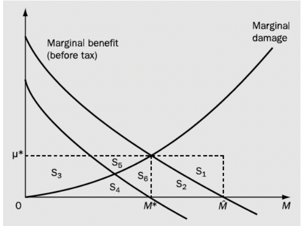
• Subsidy equals areas S1 + S2: how much is the payment? Firm loses S2, and so net gain S1.
• Tax is a loss of S3 + S4 + S5 + S6 - also lost profits on reduced output S2.

Are taxes and subsidies equivalent?

• An emissions tax and an emissions abatement subsidy (at the same rate) differ in terms of the distribution of gains and losses.
  • Different distributional effects: the burden of taxes falls on producers and consumers of the polluting product, while the burden of subsidies falls on taxpayers.
• Important implications for the political acceptability and the political feasibility of the instruments.
• It also could affect the long-run level of pollution abatement under some circumstances, via alteration of the size of the industry.
  • Subsidies raise profits to industry, and so create incentives for new firms to enter. Number of firms increases – what happens to emissions?
• Moral hazard: incentive to increase baseline emissions to earn higher subsidies.

Progressive or regressive

• Taxes may be regressive: households with lower income pay a greater share of their resources than those with higher income.
• This is a key argument in the debate about the use of carbon taxes to reduce CO2 emissions, especially direct household CO2 taxes.
• Direct CO2 tax payments → energy consumption;
• Indirect tax payments → commodities such as water, travel, various types of food.

CAC: setting up standards

• If we cannot observe MAC and MD
• Best bet is to set up a standard?
• Dominant method in most countries in the world.
• The amount of emissions depends on the goods that is produced.
• Also the technology that is used in the production process.
• Amount or mix of inputs used.

Non-transferable emissions licences

• Suppose that the EPA is committed to attaining some overall emissions target for a particular pollutant. It creates licences (also known as permits or quotas) for that total allowable quantity.
  • After adopting some criterion for apportioning licences among the individual sources, the EPA distributes licences to emissions sources.
  • These licenses are non-transferable; that is, the licences cannot be transferred (exchanged) between firms.
  • Therefore, each firm’s initial allocation of pollution licences sets the maximum amount of emissions that it is allowed.
• Successful operation of licence schemes is unlikely if polluters believe their actions are not observed, or if the penalties on polluters not meeting licence restrictions are low relative to the cost of abatement.
  • Licence schemes will have to be supported, therefore, by monitoring systems and by sufficiently harsh penalties for non-compliance.
  • This might not be cost-effective.
    • Under special conditions, the use of such emissions licences will achieve an overall target at least cost (that is, be cost-efficient).
    • But it is highly unlikely that these conditions would be satisfied.Cost-efficiency requires the marginal cost of emissions abatement to be equal over all abaters
      • If the EPA knew each polluter’s abatement cost function, it could calculate which level of emissions of each firm (and so which number of licences for each firm) would generate this equality and meet the overall target.
      • It is very unlikely that the EPA would possess, or could acquire, sufficient information to set standards for each polluter in this way.
      • The costs of collecting that information could be prohibitive, and may outweigh the potential efficiency gains arising from intervention.

Cost-efficiency

• Problem of information asymmetries; those who possess the necessary information about abatement costs at the firm level (the polluters) do not have incentives to provide it in unbiased form to those who do not have it (the regulator).
• A system of long-term relationships between regulator and regulated may partially overcome these asymmetries.
• Given all this, it seems likely that arbitrary methods will be used to allocate licences, and so the controls will not be cost-efficient.

Instruments which impose minimum technology requirements

• Command and control instruments that consist of regulations which specify required characteristics of production processes or capital equipment used.
• In other words, minimum technology requirements are imposed upon potential polluters.
• Examples of this approach have been variously known as best practicable means (BPM), best available technology (BAT) and best available technology not entailing excessive cost (BATNEEC).
• In some variants of this approach, specific techniques are mandated, such as requirements to use flue-gas desulphurisation equipment in power generation or minimum stack heights.

Cost-effectiveness

• Much the same comments about cost-effectiveness can be made for technology controls as for licences.
• They are usually not cost-efficient, because the instrument does not focus abatement effort on polluters that can abate at least cost.
• Moreover, there is an additional inefficiency here that also involves information asymmetries.
• Technology requirements restrict the choice set allowed to firms to reduce emissions.
• Decisions about emissions reduction are effectively being centralised (to the EPA) when they may be better left to the firms (who will choose this method of reducing emissions rather than any other only if it is least-cost for them to do so).
• Although technology-based instruments may be lacking in cost-effectiveness terms, they can be very powerful; they are sometimes capable of achieving large reductions in emissions quickly, particularly when technological ‘fixes’ are available but not widely adopted.
• Technology controls have almost certainly resulted in huge reductions in pollution levels compared with what would be expected in their absence

Location

• Pollution control objectives , in so far as they are concerned only with reducing human exposure to pollutants, could be met by separating the locations of people and pollution sources.
• This is only relevant where the pollutant is not uniformly mixing, so that its effects are spatially differentiated.
• Separation can be done ex ante or ex post.
• Separation ex ante, by zoning or planning control, is relatively common.
• Planning controls and other forms of direct regulation directed at location have a large role to play in the control of pollution with localised impacts and for mobile source pollution. They are also used to prevent harmful spatial clustering of emission sources.
• Ex post relocation decisions are rarer because of their draconian nature; examples include people being removed from heavily contaminated areas, such as Chernobyl.
• Location decisions of this kind will not be appropriate where we are concerned about wider ecosystem impacts or where pollution is uniformly mixing.

CAC: assessment

Attractive Properties

• Certainty of outcome.
• Ability to get desired results very quickly.

Unattractive Properties

• Likely to be cost-inefficient, as CAC techniques contain no mechanisms to bring about two desired results:
  • Equalisation of marginal abatement costs over the controlled firms in that programme.
  • Equalisation of marginal abatement costs across different programmes.
  • Lack good dynamic incentives: once standard is met firms stop.

Tradable emissions permits (inbetween CAC and market incentive instruments)

• Based on the principle that any increase in emissions must be offset by an equivalent decrease elsewhere.
• There is a limit set on the total quantity of emissions allowed, but the regulator does not attempt to determine how that total allowed quantity is allocated among individual sources.
• It can be defined as a transferable right to a common pool resource (e.g., individual transferable quotas for fishing rights).
• Our focus: tradable emission permits (TEPs) – first proposed by T. Crocker (1966) and J. Dales (1968).
• TEPs = a market-based instrument which combines elements of the three main approaches to pollution control:
  • Regulator sets the total quantity of emissions → as for CAC;
  • Plants are assigned permits (= rights to pollute) → property-rights based approach;
  • Permits can be bought and sold → economic-incentive based approach.
• 2 types: Cap and Trade and Emission Reduction Credits (ERCs).

Cap and trade permit systems

• A cap-and-trade emission permits scheme for a uniformly mixing pollutant involves:
  • A total quantity of emissions of some particular type (the ‘cap’) that is to be allowed by a specified class of actual and potential emitters over some period of time.
  • The creation of a quantity of emissions permits that in sum equal, in units of permitted emissions, to the emissions cap (the target level of emissions).
• A mechanism by which the total quantity of emission permits is initially allocated between potential polluters.
• A rule which states that no firm is allowed to emit pollution (of the designated type) beyond the quantity of emission permits it possesses.
• A system whereby actual emissions are monitored and penalties – of sufficient deterrent power – are applied to sources which emit in excess of the quantity of permits they hold.
• A guarantee that emission permits can be freely traded between firms at whichever price is agreed for that trade.
• Suppose that permits have been allocated at no charge to firms in some arbitrary way.
  • Once this initial allocation has taken place, firms will evaluate the marginal worth of permits to themselves.
  • Some firms hold more permits than the quantity of their desired emissions, and so the value of a marginal permit to these firms is zero.
  • Others hold permits in quantities insufficient for the emissions that they would have chosen in the absence of the permit system.
• The marginal valuations of permits to these firms will depend upon their emission abatement costs.
  • Some will have high marginal abatement costs, and so are willing to pay high prices to purchase emissions permits.
  • Others can abate cheaply, so that they are willing to pay only small sums to purchase permits; their marginal permit valuation is low.
• It is not necessarily the case that a firm which holds fewer permits than its desired emissions level will buy permits.
  • It always has the option available to reduce its emissions to its permitted level by undertaking extra abatement.
  • The firm may find it preferable to sell permits (rather than buy them) if the price at which they could be sold exceeds its marginal abatement cost.
• In any situation where many units of a homogeneous product are held by individuals with substantially differing marginal valuations, a market for that product will emerge.
  • In this case, the product is tradable permits, and the valuations differ because of marginal abatement cost differences between firms.
  • Therefore, a market will become established for permits, and a single, equilibrium market price will emerge, say μ.

The initial allocation of permits and the determination of the equilibrium market price of permits

• How to distribute the cap?
• Two general methods of initial allocation:
  • Case 1: the EPA sells all permits by auction.
  • Case 2: the EPA allocates all permits at no charge (which in turn requires that a distribution rule be chosen).

Conclusion

Which instrument to use?

Teacher didn’t answer, I guess it’s difficult to choose and depends on many factors.

UNIGE EnvironmentalEconomics